Create a slopegraph or bump chart from a data frame of ranks.
Usage
rankslopegraph(
  df,
  names,
  group,
  force.grouping = TRUE,
  line.size = 1,
  line.alpha = 0.5,
  line.col = NULL,
  point.size = 1,
  point.alpha = 0.5,
  point.col = NULL,
  text.size = 2,
  legend.position = "bottom"
)
Arguments
- df
A data frame of records.
- names
The name of the column having the names of the records.
- group
Optional. The name of the column with a grouping variable.
- force.grouping
If
TRUE, the column specified in the argumentnameswill be considered as a grouping variable for plotting the slopegraphs. (Each record will be represented by a different colour). Default isTRUE.- line.size
Size of lines plotted. Must be numeric.
- line.alpha
Transparency of lines plotted. Must be numeric.
- line.col
Default is
TRUE. Overrides colouring byforce.groupingargument.- point.size
Size of points plotted. Must be numeric.
- point.alpha
Transparency of points plotted. Must be numeric.
- point.col
Default is
TRUE. Overrides colouring byforce.groupingargument.- text.size
Size of text annotations plotted. Must be numeric.
- legend.position
Position of the legend in the plot.
References
Tufte ER (1986). The Visual Display of Quantitative Information. Graphics Press, Cheshire, CT, USA. ISBN 0-9613921-0-X.
Examples
library(agricolae)
data(soil)
dec <- c("pH", "EC")
inc <- c("CaCO3", "MO", "CIC", "P", "K", "sand",
"slime", "clay", "Ca", "Mg", "K2", "Na", "Al_H", "K_Mg", "Ca_Mg",
"B", "Cu", "Fe", "Mn", "Zn")
soilrank <- rankdf(soil, increasing = inc, decreasing = dec)
soilrank
#> place pH EC CaCO3 MO CIC P K sand slime clay Ca Mg K2 Na Al_H K_Mg
#> 1 Namora 13.0 7 4.5 5.0 1 3 1 13.0 2.0 1.0 1 2 2 6.5 11 11
#> 2 Hyo1 5.0 4 10.0 11.0 10 7 8 1.0 11.0 13.0 13 7 8 4.0 4 6
#> 3 Hyo2 1.5 9 13.0 8.5 8 8 7 4.5 7.0 10.5 11 10 7 1.0 4 3
#> 4 SR1 9.0 6 4.5 7.0 7 6 6 10.0 6.0 6.0 10 6 6 10.0 9 4
#> 5 SR2 11.5 8 4.5 8.5 2 2 2 12.0 1.0 3.0 2 1 1 4.0 10 12
#> 6 Cnt1 4.0 3 9.0 2.0 4 5 10 7.0 10.0 7.0 8 5 11 11.0 4 10
#> 7 Cnt2 3.0 2 12.0 5.0 12 9 13 2.0 9.0 12.0 12 12 13 12.0 4 8
#> 8 Cnt3 1.5 1 11.0 1.0 5 13 11 8.0 4.5 9.0 7 9 10 13.0 4 7
#> 9 Chz 7.0 12 4.5 3.0 3 4 5 9.0 4.5 8.0 6 4 5 8.0 4 5
#> 10 Chmar 11.5 11 4.5 12.0 13 11 9 11.0 3.0 2.0 3 3 9 6.5 13 13
#> 11 Hco1 10.0 5 4.5 10.0 9 10 3 4.5 13.0 4.5 9 13 3 9.0 8 1
#> 12 Hco2 6.0 13 4.5 5.0 6 1 4 3.0 8.0 10.5 5 11 4 2.0 4 2
#> 13 Hco3 8.0 10 4.5 13.0 11 12 12 6.0 12.0 4.5 4 8 12 4.0 12 9
#> Ca_Mg B Cu Fe Mn Zn
#> 1 7 9 1.0 7.0 2.0 2
#> 2 13 2 13.0 2.5 1.0 13
#> 3 6 5 8.5 5.0 10.0 10
#> 4 12 7 10.0 10.0 8.0 11
#> 5 10 5 2.0 9.0 3.0 1
#> 6 11 11 11.0 2.5 4.5 5
#> 7 4 12 5.0 1.0 4.5 12
#> 8 5 13 4.0 4.0 7.0 9
#> 9 9 5 6.0 8.0 13.0 6
#> 10 8 10 7.0 11.0 9.0 7
#> 11 2 8 3.0 6.0 6.0 3
#> 12 1 1 8.5 12.0 11.0 4
#> 13 3 3 12.0 13.0 12.0 8
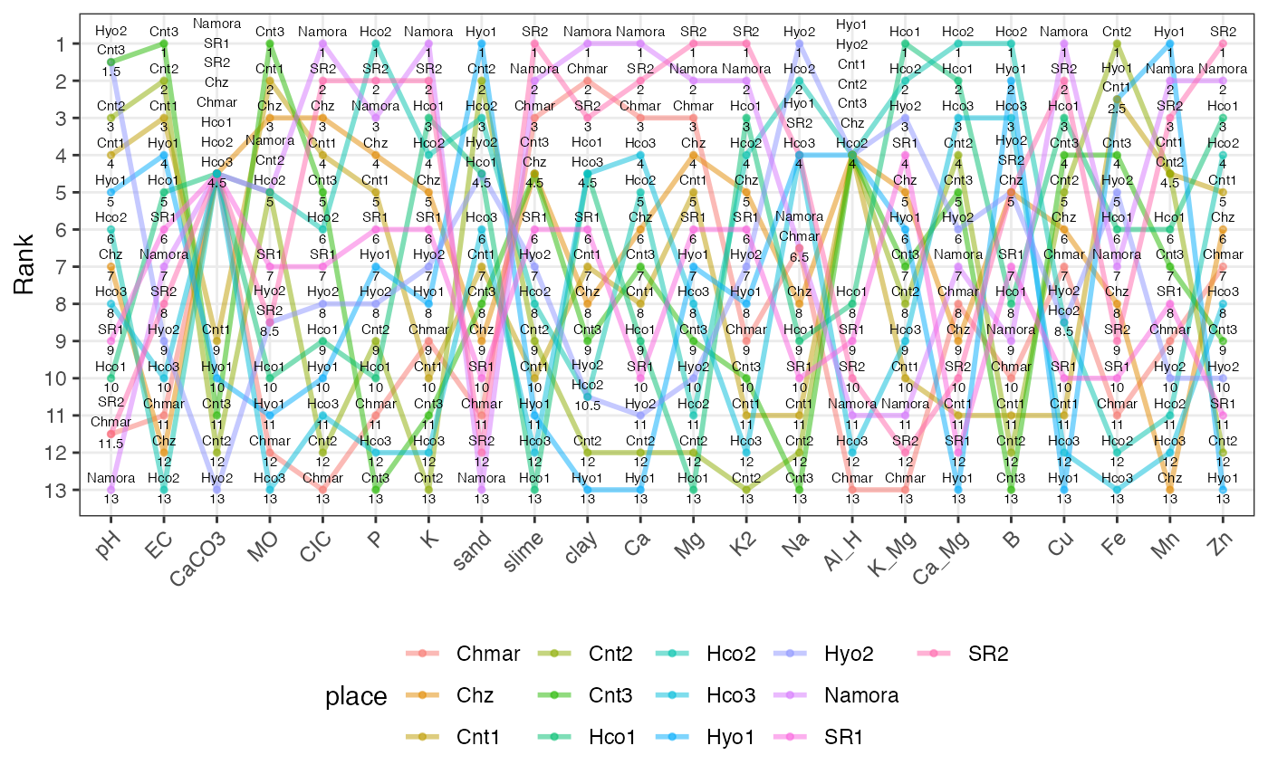
soilslopeg <- rankslopegraph(soilrank, names = "place")
soilslopeg